Detection of Cyberthreats with Computer Vision (Part 2)

Introduction 

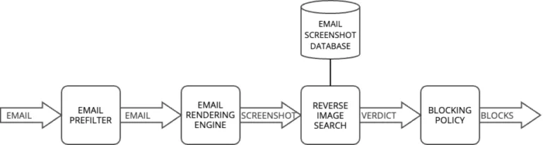
In our previous article, we explored how Computer Vision can be used to enhance cybersecurity by analyzing the visual representation of emails and webpages. We highlighted how this approach helps detect sophisticated attacks that traditional content analysis might miss. We concluded by introducing a Reverse Image Search system, which is responsible for identifying recurring malicious campaigns by comparing the screenshots of incoming emails with known threats. 

This second article in our series digs deeper into the technical challenges of detecting duplicate and near-duplicate images in a cybersecurity context. While detecting exact image duplicates might seem straightforward, attackers frequently introduce subtle variations to evade detection. A phishing campaign, for instance, might use slightly modified versions of the same template, with minor changes in colors, spacing, or embedded elements, while maintaining the same malicious intent. 

To address this challenge, we will explore two fundamental techniques for detecting images similarity: hash-based techniques and color histograms. These methods form the foundation of more sophisticated image matching systems (that will be introduced in the third article of this series) and offer different trade-offs between accuracy, performance, and resilience to various types of image modifications. 

Duplicate image detection for threat analysis 

What is a duplicate image? 

A duplicate image can be either an exact copy or a modified version of an original image. In cybersecurity campaigns, attackers often create variations of the same image through subtle modifications: rotating, resizing, adding text, or applying filters. 

While these variations look different enough to bypass security filters, they remain visually similar enough for users to recognize them as related. This creates a unique challenge: how can we automatically detect these similarities that are obvious to human eyes but complex for traditional security systems? 

How our Reverse Image Search system works 

Our Reverse Image Search system is designed to identify duplicates and variations of known malicious images. We maintain a database of known malicious email screenshots, which is used to analyze incoming emails. 

When a new email arrives, the system compares its visual rendering against this database to identify potential duplicates or variations of known threats. Rather than simply classifying images as duplicates or non-duplicates, our system calculates a similarity score between 0 and 1 for each comparison. 

This continuous scale provides more granular control over detection thresholds, allowing us to fine-tune our system’s sensitivity to match different threat scenarios. 

Blocking malicious elements 

Upon detecting a duplicate threat, our blocking policy automatically triggers defensive measures, preventing further attacks by blocking associated elements like IP addresses, URLs, and domains. 

Detection pipeline strategy 

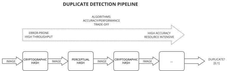
Our detection pipeline follows a progressive filtering strategy, balancing speed and accuracy. The first layers employ rapid detection techniques which, while potentially less precise, can quickly process large volumes of emails. Only the most suspicious emails proceed to more computationally intensive techniques. This funnel approach optimizes resource usage while maintaining effective threat detection. 

Reference images 

Throughout this article, we will use a consistent set of reference images to demonstrate each detection technique, making it easier to compare their effectiveness and capabilities.

The four images above will serve as reference images. Among them, images A and B are identical copies. Image C is a variant with minor text modifications in the password recovery section. Image D shows an entirely different scene.

Hash-based detection techniques 

Hash-based duplicate images detection techniques are algorithms used to identify duplicate or similar images by generating unique signatures, known as hashes, for each image. These hashes serve as compact representations of the image’s content and characteristics. 

Cryptographic hash functions 

The fundamental idea behind hash-based techniques is to convert an image into a fixed-length string of bits (hash code) in a way that similar images yield similar hash codes. As a result, exact duplicates will produce identical hash codes, making it easy to identify them efficiently. The simplest hash algorithms we can use are cryptographic functions, such as MD5 or SHA-1.  

The table below presents the MD5 hashes of the images. As expected, only exact duplicates are detected as duplicate images. This is because the cryptographic hash functions, originally designed for security and data integrity, demonstrates the Avalanche Effect: even a small change in the file results in a significantly different hash value. 

Image	MD5 hash
A (original)	fb5e836185a7b3044e0fbb729b9e5a45
B (exact duplicate)	fb5e836185a7b3044e0fbb729b9e5a45
C (near duplicate)	0adc239afeeddab5812b9630dba97883
D (different)	153f8ef8a277f9c11d4f18ba9ae6df6a

Perceptual hashing overview 

Unlike cryptographic hashes, perceptual hash techniques provide a more flexible approach that accommodates the inherent variations in images due to modifications, scaling, and other transformations. 

Perceptual hashing is a type of Locality-Sensitive Hashing (LSH), a broader class of algorithms designed for tasks like data clustering and nearest neighbor search. Unlike traditional hash functions, LSH ensures that small variations in the source data result in small variations, or no variation at all, in the hash. This property makes perceptual hashing particularly well-suited for identifying visually similar images, even when they have undergone minor transformations. 

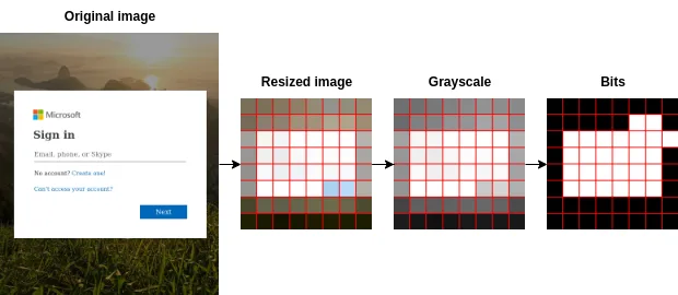
Let’s explore one of the simplest perceptual hash functions: Average Hash. 

Average Hash: A simple perceptual hashing method 

Average Hash simplifies complex images into a compact representation while retaining their essential characteristics. The steps of this technique are as follows: 

• Image Preprocessing: The image is first resized to a standard dimension (8×8 pixels, 64 total pixels). This resizing ensures uniformity in processing and minimizes the influence of small details.
• Grayscale Conversion: The resized image is then converted to grayscale. Grayscale conversion simplifies the image, making it more resilient to color variations and improving algorithm efficiency.
• Calculating Average Pixel Value: The average pixel intensity value of the grayscale image is computed. This value serves as a baseline for determining whether individual pixels are darker or lighter than the average.
• Generating Hash Code: Each pixel’s intensity is compared to the average intensity. If the pixel is brighter, it is assigned a value of 1; otherwise, it is assigned 0. These binary values are concatenated into a 64-bit integer, creating a hash code that represents the image’s distinctive visual characteristics. 

Hash comparison and similarity scoring 

The table below presents the hashes of each of the images using Average Hash function: the modified image’s hash is almost the same as the original one, except for two bits. 

Image	Average hash
A (original)	ffc7ff8181c3ffff
B (exact duplicate)	ffc7ff8181c3ffff
C (near duplicate)	ffc7ff8080c3ffff
D (different)	00067f7e7e7e0000

To compare two images, the simplest approach involves using the Hamming distance on their respective hashes. This distance measures the count of differing bit positions between the hashes. For instance, identical images yield a Hamming distance of zero. To manipulate scores, an alternative calculation is employed: 

{BEGIN SOURCE CODE} 
average_score(a, b) = 1 - (Hamming(a, b) / 64) 
{END SOURCE CODE} 

This formula offers a convenient scale from 0 to 1, where 0 signifies entirely dissimilar images, and 1 indicates exact duplicates. The following table displays the Hamming distances and corresponding scores with the original image. Subsequently, it only requires establishing a threshold value above which two images are classified as duplicates. 

Image	Hamming distance to Image A	Score distance to Image A
B (exact duplicate)	0	1.000
C (near duplicate)	2	0.969
D (different)	50	0.219

Limitations of perceptual hashing 

While effective in detecting exact or near duplicates, perceptual hashes might have difficulties with altered images, with transformations such as rotation or scaling. 

Additionally, perceptual hashing methods might occasionally yield false positives or negatives, impacting accuracy, especially when dealing with images that share similar visual elements but have different semantic content. For example, Hao et al. proposed in “It’s Not What It Looks Like: Manipulating Perceptual Hashing based Applications” a series of attack algorithms to subvert perceptual hashing techniques. 

To address these limitations, perceptual hashing is often combined with content-based techniques, such as color histograms, presented in the next section. 

Color histograms 

An inherent limitation of the average hash technique previously presented is its disregard for image color due to its grayscale nature. Therefore, a promising avenue for enhancing our system involves implementing a content-based approach that centers exclusively on colors, utilizing color histograms.

This approach revolves around capturing the distribution of colors present in an image and representing it as a histogram. By quantifying the occurrence of each color in the image, the color histogram technique offers a powerful tool for identifying images with similar color patterns. 

From an image to histograms 

Computing color histograms from an image involves several steps: 

• Image preparation: Convert the image into a convenient RGB color space and resize it to a smaller size for performance reasons. 
• Quantization: Reduce the number of distinct colors in the image while retaining its overall visual quality. This helps us save memory and reduce computational complexity. We use a reduced color palette of 16 colors, designed for a variety of tasks. 

• Counting pixels: Count the number of pixels that fall within each of the 16 color buckets.
• Normalization: To ensure that histograms are independent of the image’s size, we normalize the values by dividing the count of pixels of each color by the total number of pixels in the image.

To ease the comprehension of this technique, the chart below displays partial color histograms for the four images, showcasing only four of the sixteen colors.

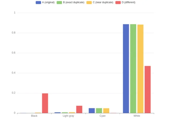
Histogram comparison and similarity scoring

Similar to the approach used for hashes, we calculate the distances between the color histograms using the Manhattan distance – also referred to as the L1 distance – that involves calculating the sum of absolute differences between values in the histograms. When employing this distance to compare images, similar color distributions will yield smaller distances. In the opposite extreme case, where two histograms are completely different, the L1 distance is 2 (the sum of the two normalized histograms). As done previously for the average score, we prefer an alternative calculation.

{BEGIN SOURCE CODE} 
L1_dist(a, b) = abs(a[0] - b[0]) + abs(a[1] - b[1]) + ... + abs(a[15] - b[15]) 
hist_score(a, b) = 1 – L1_dist(a, b) / 2 
{END SOURCE CODE} 

This formula offers a convenient scale from 0 to 1, where 0 signifies entirely dissimilar image color distribution, and 1 indicates the exact same color distribution. The following table displays the L1 distance and histogram scores with the original image. 

Image	L1 distance to Image A	Score distance to Image A
B (exact duplicate)	0.000	1.000
C (near duplicate)	0.011	0.994
D (different)	1.024	0.488

Limitations of color histograms 

This approach has a clear limitation: it solely examines the distribution of colors within images, without considering their location. Also, we have to be careful about the size of the reduced color palette, that could have an impact on the results. While the techniques covered thus far – including perceptual hashing and color histograms – might indicate image resemblances, it’s crucial to verify whether the depicted objects are truly similar. This aspect will be the subject of the next article. 

---

---

Conclusion 

In this article, we explored two fundamental techniques for detecting duplicate and near-duplicate images: hash-based methods and color histograms. While these approaches offer efficient initial filtering capabilities, they each have their limitations. Perceptual hashing can be vulnerable to specific alterations, and color histograms, while useful for analyzing color distributions, do not consider the spatial arrangement of visual elements. 

These techniques serve well as rapid screening mechanisms in our detection pipeline, offering a good balance between computational efficiency and approximate matching. However, for high-stakes security decisions, we need more sophisticated methods to verify that detected similarities truly indicate duplicate threats. 

In our next article, we will explore content-based approaches that analyze the actual visual elements and their relationships within images. These methods, while more computationally intensive, provide the high accuracy needed for reliable duplicate detection. We will examine how these techniques can help us confidently identify variants of known threats, even when attackers employ sophisticated modification techniques to evade detection. 

---

---